SUEWS Quick Start Tutorial

3.1.1. SUEWS Quick Start Tutorial#

This tutorial demonstrates the essential SUEWS workflow using the modern SuPy (Python) interface:

Load sample data
Run simulation
Explore results

3.1.1.1. What is SUEWS?#

SUEWS (Surface Urban Energy and Water Balance Scheme) is an urban climate model that simulates energy and water fluxes in urban environments. SuPy is the modern Python interface that provides powerful data analysis capabilities and seamless integration with the scientific Python ecosystem.

Key Benefits of SuPy: - Modern YAML configuration: Type-safe, hierarchical parameter organization - pandas integration: Powerful data analysis and visualization - Scientific Python ecosystem: Works with NumPy, matplotlib, Jupyter notebooks - Built-in sample data: Start immediately without complex setup

3.1.1.2. Installation#

Install SuPy with one command:

pip install supy

3.1.1.3. Before We Start#

Load the necessary packages:

[1]:

import matplotlib.pyplot as plt
import supy as sp
import pandas as pd
import numpy as np
from pathlib import Path

%matplotlib inline

[2]:

sp.show_version()

2025.11.19.dev7

3.1.1.4. Load Sample Data#

SuPy includes built-in sample data to get you started immediately. This is the recommended approach for learning SUEWS and testing functionality.

3.1.1.4.1. Recommended Approach: Built-in Sample Data#

Load sample data for immediate simulation. This approach provides built-in test data and configurations, perfect for learning and testing:

[4]:

# Load built-in sample data using modern OOP API
from supy import SUEWSSimulation as ss

sim_sample = ss.from_sample_data()

# Extract state and forcing for examination
df_state_init = sim_sample.state_init
df_forcing = sim_sample.forcing

# Examine the sample data
print(" Sample data loaded successfully!")
print(f"Grid ID: {df_state_init.index[0]}")
print(f"Forcing period: {df_forcing.index[0]} to {df_forcing.index[-1]}")
print(f"Time steps: {len(df_forcing)}")

# For demonstration, use one year of data
df_forcing = df_forcing.loc["2012"].iloc[1:]
grid = df_state_init.index[0]

2025-11-19 23:45:56,771 - SuPy - INFO - Loading config from yaml
 Sample data loaded successfully!
Grid ID: 1
Forcing period: 2012-01-01 00:05:00 to 2013-01-01 00:00:00
Time steps: 105408

A sample df_state_init looks below (note that .T is used here to produce a nicer tableform view):

3.1.1.4.2. Alternative: Complete Simulation in One Step#

For even simpler usage, you can run a complete simulation with sample data in one command:

Run complete simulation with sample data in one step

sim = SUEWSSimulation.from_sample_data()
sim.run()
df_output, df_state_final, df_forcing = sim.results, sim.df_state_final, sim.df_forcing

This approach is ideal for: - Quick testing and demonstration - Learning SUEWS output structure - Benchmarking performance

For this tutorial, we’ll use the step-by-step approach above for better learning

3.1.1.4.3. Understanding the Input Data#

SUEWS requires two main input datasets:

3.1.1.4.3.1. `df_state_init` - Initial Conditions and Site Configuration#

df_state_init contains: - Surface characteristics: albedo, emissivity, land cover fractions, building heights - Model configuration: physics options, time stepping, output settings

For complete variable descriptions, see Input Data Structures

[7]:

df_state_init.loc[:, ["bldgh", "evetreeh", "dectreeh"]]

[7]:

var	bldgh	evetreeh	dectreeh
ind_dim	0	0	0
grid
1	22.0	13.1	13.1

[8]:

df_state_init.filter(like="sfr_surf")

[8]:

var	sfr_surf
ind_dim	(0,)	(1,)	(2,)	(3,)	(4,)	(5,)	(6,)
grid
1	0.43	0.38	0.0	0.02	0.03	0.0	0.14

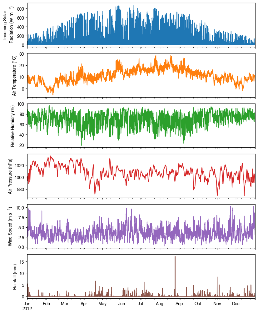
3.1.1.4.3.2. `df_forcing` - Meteorological Forcing Data#

df_forcing contains time series of meteorological variables that drive the urban climate simulation.

For complete variable descriptions, see Input Data Structures.

Below is an overview of the key forcing variables in our sample dataset:

[9]:

list_var_forcing = [
    "kdown",
    "Tair",
    "RH",
    "pres",
    "U",
    "rain",
]
dict_var_label = {
    "kdown": "Incoming Solar\n Radiation ($ \mathrm{W \ m^{-2}}$)",
    "Tair": "Air Temperature ($^{\circ}$C)",
    "RH": r"Relative Humidity (%)",
    "pres": "Air Pressure (hPa)",
    "rain": "Rainfall (mm)",
    "U": "Wind Speed (m $\mathrm{s^{-1}}$)",
}
df_plot_forcing_x = (
    df_forcing.loc[:, list_var_forcing].copy().shift(-1).dropna(how="any")
)
df_plot_forcing = df_plot_forcing_x.resample("1h").mean()
df_plot_forcing["rain"] = df_plot_forcing_x["rain"].resample("1h").sum()

axes = df_plot_forcing.plot(
    subplots=True,
    figsize=(8, 12),
    legend=False,
)
fig = axes[0].figure
fig.tight_layout()
fig.autofmt_xdate(bottom=0.2, rotation=0, ha="center")
for ax, var in zip(axes, list_var_forcing):
    _ = ax.set_ylabel(dict_var_label[var])

../../_images/tutorials_python_quick-start_13_0.png

3.1.1.4.4. Modifying Input Data#

Since SuPy uses pandas DataFrames, you can easily modify input parameters using standard pandas operations. This is useful for sensitivity analyses or site-specific adjustments:

Given pandas.DataFrame is the core data structure of SuPy, all operations, including modification, output, demonstration, etc., on SuPy inputs (df_state_init and df_forcing) can be done using pandas-based functions/methods.

Specifically, for modification, the following operations are essential:

3.1.1.4.4.1. Locating Parameters#

Data can be located in two ways: 1. By name using `.loc <http://pandas.pydata.org/pandas-docs/stable/user_guide/indexing.html#selection-by-label>`__ 2. By position using `.iloc <http://pandas.pydata.org/pandas-docs/stable/user_guide/indexing.html#selection-by-position>`__

Data can be located in two ways, namely: 1. by name via `.loc <http://pandas.pydata.org/pandas-docs/stable/user_guide/indexing.html#selection-by-label>`__; 2. by position via `.iloc <http://pandas.pydata.org/pandas-docs/stable/user_guide/indexing.html#selection-by-position>`__.

[10]:

# view the surface fraction variable: `sfr`
df_state_init.loc[:, "sfr_surf"]

[10]:

ind_dim	(0,)	(1,)	(2,)	(3,)	(4,)	(5,)	(6,)
grid
1	0.43	0.38	0.0	0.02	0.03	0.0	0.14

[11]:

# view the second row of `df_forcing`, which is a pandas Series
df_forcing.iloc[1]

[11]:

iy       2012.00
id          1.00
it          0.00
imin       15.00
qn       -999.00
qh       -999.00
qe       -999.00
qs       -999.00
qf       -999.00
U           4.61
RH         85.47
Tair       11.77
pres     1001.50
rain        0.00
kdown       0.16
snow     -999.00
ldown    -999.00
fcld     -999.00
Wuh         0.00
xsmd     -999.00
lai      -999.00
kdiff    -999.00
kdir     -999.00
wdir     -999.00
isec        0.00
Name: 2012-01-01 00:15:00, dtype: float64

[12]:

# view a particular position of `df_forcing`, which is a value
df_forcing.iloc[8, 9]

[12]:

np.float64(4.61)

3.1.1.4.4.2. Modifying Parameters#

Setting new values is straightforward. After locating the variables to modify, simply assign new values:

Setting new values is very straightforward: after locating the variables/data to modify, just set the new values accordingly:

[13]:

# modify surface fractions
df_state_init.loc[:, "sfr_surf"] = [0.1, 0.1, 0.2, 0.3, 0.25, 0.05, 0]
# check the updated values
df_state_init.loc[:, "sfr_surf"]

[13]:

ind_dim	(0,)	(1,)	(2,)	(3,)	(4,)	(5,)	(6,)
grid
1	0.1	0.1	0.2	0.3	0.25	0.05	0

3.1.1.5. Run Simulation#

Once forcing data (df_forcing) and initial conditions (df_state_init) are ready, call sim.run() to perform the SUEWS simulation. This stores results accessible via sim.results (or sim.df_output) and sim.df_state_final.

Once met-forcing (via df_forcing) and initial conditions (via df_state_init) are loaded in, we call sim.run() to conduct a SUEWS simulation, which will return two pandas DataFrames: df_output and df_state.

[16]:

# Run simulation
sim_sample.run()

# Access results
df_output = sim_sample.results
df_state_final = sim_sample.state_final

[16]:

	group	BEERS										...	SUEWS
	var	azimuth	altitude	GlobalRad	DiffuseRad	DirectRad	Kdown2d	Kup2d	Ksouth	Kwest	Knorth	...	Ts_Grass	Ts_BSoil	Ts_Water	Ts_Paved_dyohm	Ts_Bldgs_dyohm	Ts_EveTr_dyohm	Ts_DecTr_dyohm	Ts_Grass_dyohm	Ts_BSoil_dyohm	Ts_Water_dyohm
grid	datetime
1	2012-01-01 00:05:00	0.931142	-61.632826	0.16	0.0	0.0	0.0	0.0	0.0	0.0	0.0	...	12.870186	12.864744	12.862176	10.900448	10.972911	10.972911	10.972911	10.972911	10.972911	10.972911
	2012-01-01 00:10:00	3.347077	-61.603569	0.16	0.0	0.0	0.0	0.0	0.0	0.0	0.0	...	12.878201	12.872726	12.870134	10.818824	10.818380	10.918016	10.918016	10.858234	10.877112	10.877112
	2012-01-01 00:15:00	5.756736	-61.541631	0.16	0.0	0.0	0.0	0.0	0.0	0.0	0.0	...	12.869776	12.864282	12.861666	10.741024	10.678091	10.865010	10.865010	10.751578	10.786983	10.786983
	2012-01-01 00:20:00	8.155703	-61.447237	0.16	0.0	0.0	0.0	0.0	0.0	0.0	0.0	...	12.853404	12.847896	12.845258	10.666848	10.550664	10.813818	10.813818	10.652340	10.702157	10.702157
	2012-01-01 00:25:00	10.539714	-61.320723	0.16	0.0	0.0	0.0	0.0	0.0	0.0	0.0	...	12.833235	12.827717	12.825055	10.596105	10.434849	10.764369	10.764369	10.559964	10.622291	10.622291
	...	...	...	...	...	...	...	...	...	...	...	...	...	...	...	...	...	...	...	...	...	...
	2012-12-31 23:40:00	348.749128	-61.223782	0.00	0.0	0.0	0.0	0.0	0.0	0.0	0.0	...	10.199067	10.818435	10.898584	6.309914	2.748652	9.184894	9.184894	3.743662	4.834199	4.834199
	2012-12-31 23:45:00	351.124899	-61.359370	0.00	0.0	0.0	0.0	0.0	0.0	0.0	0.0	...	10.185470	10.795352	10.873958	6.308790	2.747566	9.183812	9.183812	3.742610	4.833165	4.833165
	2012-12-31 23:50:00	353.516761	-61.463000	0.00	0.0	0.0	0.0	0.0	0.0	0.0	0.0	...	10.171681	10.772212	10.849304	6.307717	2.746568	9.182768	9.182768	3.741625	4.832188	4.832188
	2012-12-31 23:55:00	355.920524	-61.534305	0.00	0.0	0.0	0.0	0.0	0.0	0.0	0.0	...	10.135518	10.721713	10.796548	6.306691	2.745648	9.181761	9.181761	3.740701	4.831263	4.831263
	2013-01-01 00:00:00	358.339872	-61.573100	0.00	0.0	0.0	0.0	0.0	0.0	0.0	0.0	...	10.110590	10.685309	10.758330	6.305708	2.744798	9.180787	9.180787	3.739834	4.830386	4.830386

105408 rows × 1036 columns

3.1.1.5.1. Understanding the Output#

3.1.1.5.1.1. `df_output` - Simulation Results#

df_output contains comprehensive SUEWS output organized into groups:

SUEWS: Essential surface energy and water balance variables
DailyState: Daily aggregated state information
Snow: Snow-related variables (when snow module is active)
RSL: Rough sublayer scheme outputs
debug: Debugging information

For complete variable descriptions, see Output Data Structures

[17]:

df_output.columns.levels[0]

[17]:

Index(['BEERS', 'DailyState', 'debug', 'EHC', 'NHood', 'RSL', 'snow',
       'SPARTACUS', 'STEBBS', 'SUEWS'],
      dtype='object', name='group')

3.1.1.5.1.2. `df_state_final` - Final Model State#

df_state_final contains the model state at simulation end (or all states if save_state=True):

Same structure as df_state_init for continuity
Can be used as initial conditions for subsequent simulations
Essential for spin-up procedures and long-term studies

For complete variable descriptions, see Output Data Structures

[18]:

df_state_final.T.head()

[18]:

	datetime	2012-01-01 00:05:00	2013-01-01 00:05:00
	grid	1	1
var	ind_dim
ah_min	(0,)	15.0	15.0
ah_min	(1,)	15.0	15.0
ah_slope_cooling	(0,)	2.7	2.7
ah_slope_cooling	(1,)	2.7	2.7
ah_slope_heating	(0,)	2.7	2.7

3.1.1.6. Explore Results#

Thanks to pandas integration and the PyData ecosystem, SuPy enables powerful analysis of SUEWS results through statistics, resampling, visualization, and much more.

Thanks to the functionality inherited from pandas and other packages under the PyData stack, compared with the standard SUEWS simulation workflow, supy enables more convenient examination of SUEWS results by statistics calculation, resampling, plotting (and many more).

3.1.1.6.1. Output Data Structure#

df_output uses MultiIndex for both rows and columns: - Index: (grid, datetime) for spatial and temporal organization - Columns: (group, variable) for organized output groups

[19]:

df_output.head()

[19]:

	group	BEERS										...	SUEWS
	var	azimuth	altitude	GlobalRad	DiffuseRad	DirectRad	Kdown2d	Kup2d	Ksouth	Kwest	Knorth	...	Ts_Grass	Ts_BSoil	Ts_Water	Ts_Paved_dyohm	Ts_Bldgs_dyohm	Ts_EveTr_dyohm	Ts_DecTr_dyohm	Ts_Grass_dyohm	Ts_BSoil_dyohm	Ts_Water_dyohm
grid	datetime
1	2012-01-01 00:05:00	0.931142	-61.632826	0.16	0.0	0.0	0.0	0.0	0.0	0.0	0.0	...	12.870186	12.864744	12.862176	10.900448	10.972911	10.972911	10.972911	10.972911	10.972911	10.972911
	2012-01-01 00:10:00	3.347077	-61.603569	0.16	0.0	0.0	0.0	0.0	0.0	0.0	0.0	...	12.878201	12.872726	12.870134	10.818824	10.818380	10.918016	10.918016	10.858234	10.877112	10.877112
	2012-01-01 00:15:00	5.756736	-61.541631	0.16	0.0	0.0	0.0	0.0	0.0	0.0	0.0	...	12.869776	12.864282	12.861666	10.741024	10.678091	10.865010	10.865010	10.751578	10.786983	10.786983
	2012-01-01 00:20:00	8.155703	-61.447237	0.16	0.0	0.0	0.0	0.0	0.0	0.0	0.0	...	12.853404	12.847896	12.845258	10.666848	10.550664	10.813818	10.813818	10.652340	10.702157	10.702157
	2012-01-01 00:25:00	10.539714	-61.320723	0.16	0.0	0.0	0.0	0.0	0.0	0.0	0.0	...	12.833235	12.827717	12.825055	10.596105	10.434849	10.764369	10.764369	10.559964	10.622291	10.622291

5 rows × 1036 columns

3.1.1.6.2. Working with SUEWS Output#

We’ll focus on the essential SUEWS output group, which contains the main surface energy and water balance variables. The MultiIndex structure allows for powerful data selection and analysis:

[20]:

df_output_suews = df_output["SUEWS"]

3.1.1.6.3. Statistical Analysis#

Use the .describe() method for quick overview of key energy balance components:

[21]:

df_output_suews.loc[:, ["QN", "QS", "QH", "QE", "QF"]].describe()

[21]:

var	QN	QS	QH	QE	QF
count	105408.000000	105408.000000	105408.000000	105408.000000	105408.000000
mean	39.841331	4.782061	75.036458	44.877688	84.854876
std	131.960919	43.124399	75.610215	55.890629	32.926429
min	-86.331686	-50.028263	-132.514514	0.088436	31.148865
25%	-42.499253	-27.242348	22.828886	1.233782	53.835755
50%	-25.756024	-7.833824	54.363213	20.270206	88.340645
75%	74.772812	16.669760	111.985158	72.722885	113.242338
max	679.848644	206.186682	412.005934	371.049669	161.706726

3.1.1.6.4. Visualization#

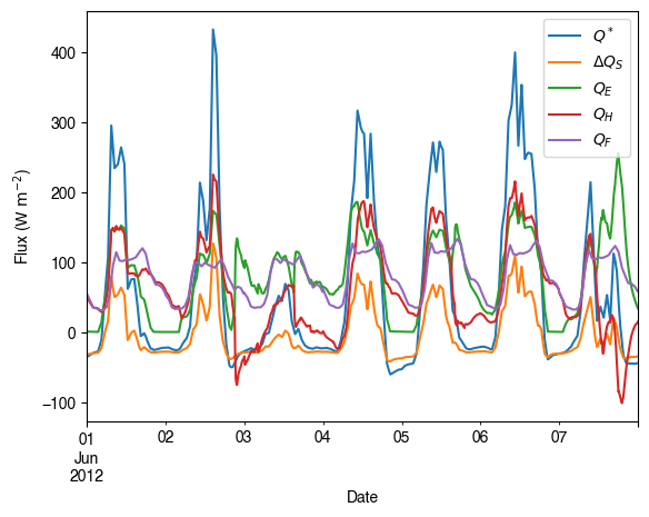
3.1.1.6.4.1. Quick Plotting Example#

Plotting is straightforward using pandas’ built-in .plot() method. Here we examine surface energy balance for one week in June:

3.1.1.6.4.2. Basic example#

Plotting is very straightforward via the .plot method bounded with pandas.DataFrame. Note the usage of loc for two slices of the output DataFrame.

[22]:

# a dict for better display variable names
dict_var_disp = {
    "QN": "$Q^*$",
    "QS": r"$\Delta Q_S$",
    "QE": "$Q_E$",
    "QH": "$Q_H$",
    "QF": "$Q_F$",
    "Kdown": r"$K_{\downarrow}$",
    "Kup": r"$K_{\uparrow}$",
    "Ldown": r"$L_{\downarrow}$",
    "Lup": r"$L_{\uparrow}$",
    "Rain": "$P$",
    "Irr": "$I$",
    "Evap": "$E$",
    "RO": "$R$",
    "TotCh": "$\Delta S$",
}

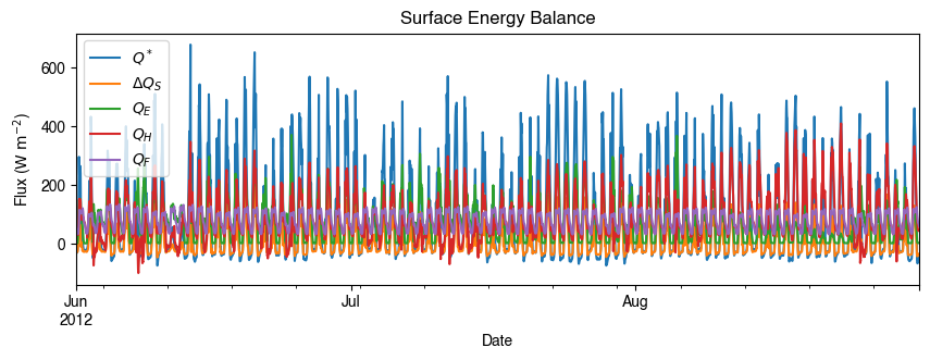
3.1.1.6.4.3. Complete Summer Analysis#

Let’s examine the full summer period (June-August) urban energy balance:

[23]:

ax_output = (
    df_output_suews.loc[grid]
    .loc["2012 6 1":"2012 6 7", ["QN", "QS", "QE", "QH", "QF"]]
    .rename(columns=dict_var_disp)
    .plot()
)
_ = ax_output.set_xlabel("Date")
_ = ax_output.set_ylabel("Flux ($ \mathrm{W \ m^{-2}}$)")
_ = ax_output.legend()

../../_images/tutorials_python_quick-start_43_0.png

3.1.1.6.4.4. More examples#

Below is a more complete example for examination of urban energy balance over the whole summer (June to August).

[24]:

# energy balance
ax_output = (
    df_output_suews.loc[grid]
    .loc["2012 6":"2012 8", ["QN", "QS", "QE", "QH", "QF"]]
    .rename(columns=dict_var_disp)
    .plot(
        figsize=(10, 3),
        title="Surface Energy Balance",
    )
)
_ = ax_output.set_xlabel("Date")
_ = ax_output.set_ylabel("Flux ($ \mathrm{W \ m^{-2}}$)")
_ = ax_output.legend()

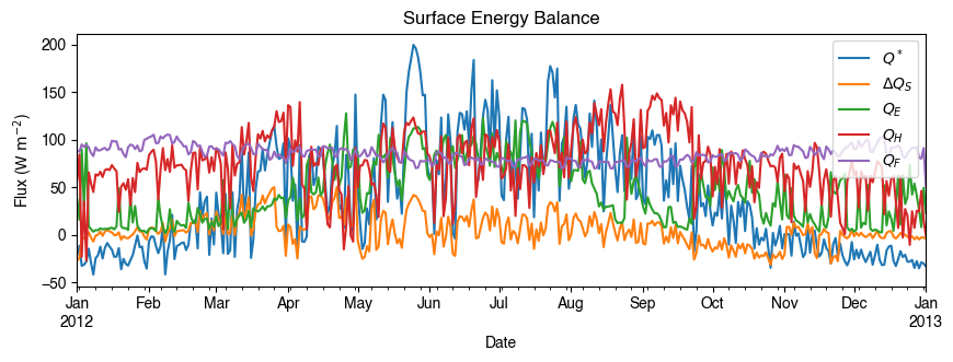
../../_images/tutorials_python_quick-start_45_0.png

3.1.1.6.5. Temporal Resampling#

SUEWS typically runs at 5-minute intervals, producing large datasets. Resampling to hourly or daily values improves analysis performance and reveals temporal patterns:

[25]:

rsmp_1d = df_output_suews.loc[grid].resample("1d")
# daily mean values
df_1d_mean = rsmp_1d.mean()
# daily sum values
df_1d_sum = rsmp_1d.sum()

3.1.1.6.5.1. Daily Mean Energy Balance#

Using daily averages makes plotting faster and reveals seasonal patterns:

[26]:

# energy balance
ax_output = (
    df_1d_mean.loc[:, ["QN", "QS", "QE", "QH", "QF"]]
    .rename(columns=dict_var_disp)
    .plot(
        figsize=(10, 3),
        title="Surface Energy Balance",
    )
)
_ = ax_output.set_xlabel("Date")
_ = ax_output.set_ylabel("Flux ($ \mathrm{W \ m^{-2}}$)")
_ = ax_output.legend()

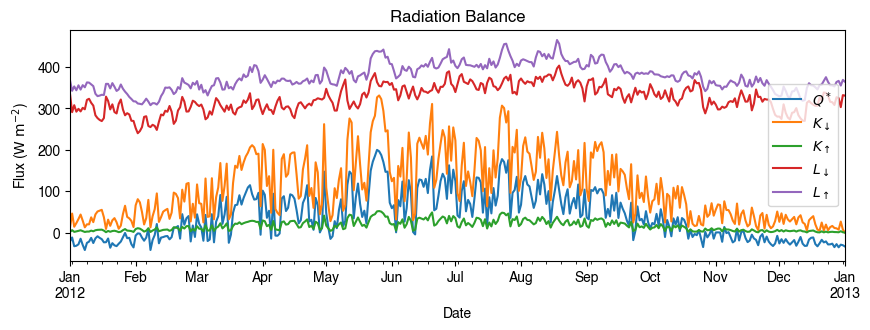
../../_images/tutorials_python_quick-start_49_0.png

3.1.1.6.5.2. Multi-Component Analysis#

Using the resampled data, we can examine both energy and water balance components:

[27]:

# radiation balance
ax_output = (
    df_1d_mean.loc[:, ["QN", "Kdown", "Kup", "Ldown", "Lup"]]
    .rename(columns=dict_var_disp)
    .plot(
        figsize=(10, 3),
        title="Radiation Balance",
    )
)
_ = ax_output.set_xlabel("Date")
_ = ax_output.set_ylabel("Flux ($ \mathrm{W \ m^{-2}}$)")
_ = ax_output.legend()

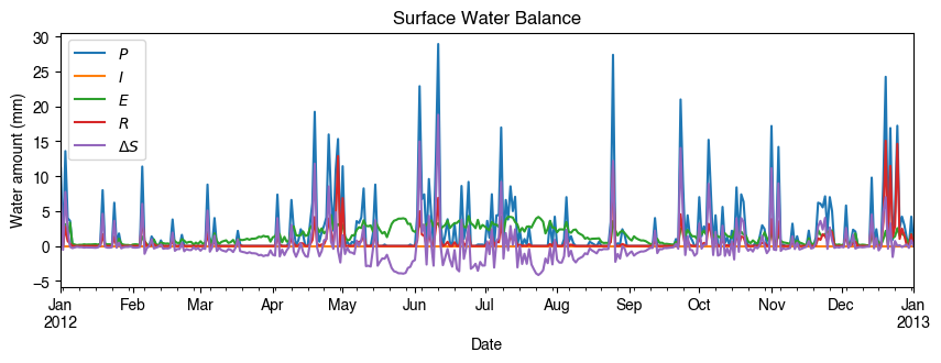
../../_images/tutorials_python_quick-start_51_0.png

[28]:

# water balance
ax_output = (
    df_1d_sum.loc[:, ["Rain", "Irr", "Evap", "RO", "TotCh"]]
    .rename(columns=dict_var_disp)
    .plot(
        figsize=(10, 3),
        title="Surface Water Balance",
    )
)
_ = ax_output.set_xlabel("Date")
_ = ax_output.set_ylabel("Water amount (mm)")
_ = ax_output.legend()

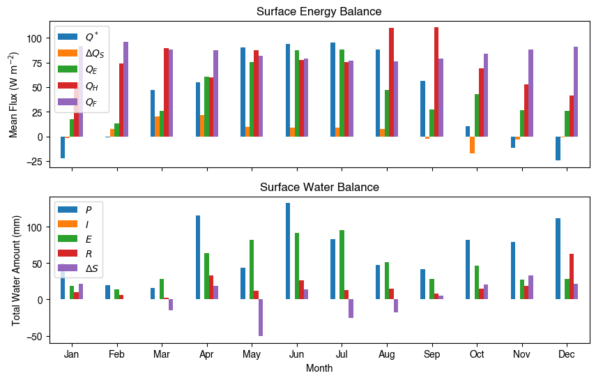
../../_images/tutorials_python_quick-start_52_0.png

3.1.1.6.5.3. Monthly Patterns#

Get an overview of seasonal energy and water balance patterns:

[29]:

# get a monthly Resampler
df_plot = df_output_suews.loc[grid].copy()
df_plot.index = df_plot.index.set_names("Month")
rsmp_1M = df_plot.shift(-1).dropna(how="all").resample("1M", kind="period")
# mean values
df_1M_mean = rsmp_1M.mean()
# sum values
df_1M_sum = rsmp_1M.sum()

[33]:

# month names
name_mon = [x.strftime("%b") for x in rsmp_1M.groups]
# create subplots showing two panels together
fig, axes = plt.subplots(2, 1, sharex=True)
# surface energy balance
_ = (
    df_1M_mean.loc[:, ["QN", "QS", "QE", "QH", "QF"]]
    .rename(columns=dict_var_disp)
    .plot(
        ax=axes[0],  # specify the axis for plotting
        figsize=(10, 6),  # specify figure size
        title="Surface Energy Balance",
        kind="bar",
    )
)
# surface water balance
_ = (
    df_1M_sum.loc[:, ["Rain", "Irr", "Evap", "RO", "TotCh"]]
    .rename(columns=dict_var_disp)
    .plot(
        ax=axes[1],  # specify the axis for plotting
        title="Surface Water Balance",
        kind="bar",
    )
)

# annotations
_ = axes[0].set_ylabel("Mean Flux ($ \mathrm{W \ m^{-2}}$)")
_ = axes[0].legend()
_ = axes[1].set_xlabel("Month")
_ = axes[1].set_ylabel("Total Water Amount (mm)")
_ = axes[1].xaxis.set_ticklabels(name_mon, rotation=0)
_ = axes[1].legend()

../../_images/tutorials_python_quick-start_55_0.png

3.1.1.6.6. Saving Results#

SuPy provides convenient functions to save output in various formats for further analysis:

The SUEWSSimulation.save() function exports results to standard text files compatible with other analysis tools:

[34]:

df_output

[34]:

	group	BEERS										...	SUEWS
	var	azimuth	altitude	GlobalRad	DiffuseRad	DirectRad	Kdown2d	Kup2d	Ksouth	Kwest	Knorth	...	Ts_Grass	Ts_BSoil	Ts_Water	Ts_Paved_dyohm	Ts_Bldgs_dyohm	Ts_EveTr_dyohm	Ts_DecTr_dyohm	Ts_Grass_dyohm	Ts_BSoil_dyohm	Ts_Water_dyohm
grid	datetime
1	2012-01-01 00:05:00	0.931142	-61.632826	0.16	0.0	0.0	0.0	0.0	0.0	0.0	0.0	...	12.870186	12.864744	12.862176	10.900448	10.972911	10.972911	10.972911	10.972911	10.972911	10.972911
	2012-01-01 00:10:00	3.347077	-61.603569	0.16	0.0	0.0	0.0	0.0	0.0	0.0	0.0	...	12.878201	12.872726	12.870134	10.818824	10.818380	10.918016	10.918016	10.858234	10.877112	10.877112
	2012-01-01 00:15:00	5.756736	-61.541631	0.16	0.0	0.0	0.0	0.0	0.0	0.0	0.0	...	12.869776	12.864282	12.861666	10.741024	10.678091	10.865010	10.865010	10.751578	10.786983	10.786983
	2012-01-01 00:20:00	8.155703	-61.447237	0.16	0.0	0.0	0.0	0.0	0.0	0.0	0.0	...	12.853404	12.847896	12.845258	10.666848	10.550664	10.813818	10.813818	10.652340	10.702157	10.702157
	2012-01-01 00:25:00	10.539714	-61.320723	0.16	0.0	0.0	0.0	0.0	0.0	0.0	0.0	...	12.833235	12.827717	12.825055	10.596105	10.434849	10.764369	10.764369	10.559964	10.622291	10.622291
	...	...	...	...	...	...	...	...	...	...	...	...	...	...	...	...	...	...	...	...	...	...
	2012-12-31 23:40:00	348.749128	-61.223782	0.00	0.0	0.0	0.0	0.0	0.0	0.0	0.0	...	10.199067	10.818435	10.898584	6.309914	2.748652	9.184894	9.184894	3.743662	4.834199	4.834199
	2012-12-31 23:45:00	351.124899	-61.359370	0.00	0.0	0.0	0.0	0.0	0.0	0.0	0.0	...	10.185470	10.795352	10.873958	6.308790	2.747566	9.183812	9.183812	3.742610	4.833165	4.833165
	2012-12-31 23:50:00	353.516761	-61.463000	0.00	0.0	0.0	0.0	0.0	0.0	0.0	0.0	...	10.171681	10.772212	10.849304	6.307717	2.746568	9.182768	9.182768	3.741625	4.832188	4.832188
	2012-12-31 23:55:00	355.920524	-61.534305	0.00	0.0	0.0	0.0	0.0	0.0	0.0	0.0	...	10.135518	10.721713	10.796548	6.306691	2.745648	9.181761	9.181761	3.740701	4.831263	4.831263
	2013-01-01 00:00:00	358.339872	-61.573100	0.00	0.0	0.0	0.0	0.0	0.0	0.0	0.0	...	10.110590	10.685309	10.758330	6.305708	2.744798	9.180787	9.180787	3.739834	4.830386	4.830386

105408 rows × 1036 columns

[36]:

# Save using OOP approach
list_path_save = sim_sample.save("output/")

3.1.1.7. Next Steps#

Congratulations! You’ve completed your first SUEWS urban climate simulation. Here’s where to go next:

3.1.1.7.1. Advanced Tutorials#

Setup Your Own Site: Configure SUEWS for your research location
Impact Studies: Climate change and scenario analysis

3.1.1.7.2. Configuration and Data#

Data Structures Guide: Detailed input/output documentation
YAML Configuration: Modern parameter management
Command-line wizard: A configuration wizard tool is in development

3.1.1.7.3. ️ Urban Climate Science#

Physical Principles: Understanding SUEWS physics
Recent Publications: Latest SUEWS research applications

3.1.1.7.4. Key Concepts You’ve Learned#

Loading sample data for immediate simulation
Running SUEWS urban climate simulations
Understanding energy balance components (QN, QH, QE, QS, QF)
Data analysis with pandas integration
Visualization and temporal resampling
Saving results for further analysis

3.1.1.7.5. Real Research Applications#

This tutorial used sample data, but SuPy enables sophisticated urban climate research: - Urban heat island studies across different cities - Climate change impact assessment for urban areas - Building energy modeling integration - Multi-site comparative studies with parallel processing - Policy scenario analysis for urban planning

Ready to apply SUEWS to your research? Start with Setup Your Own Site!

[37]:

# Display saved files
for file_out in list_path_save:
    print(f" {file_out.name}")

print("\n Congratulations! You've completed your first SUEWS simulation.")
print(" Results saved in multiple formats for further analysis.")
print(" Ready for more advanced applications!")

 KCL1_2012_SUEWS_60.txt
 df_state_KCL.csv

 Congratulations! You've completed your first SUEWS simulation.
 Results saved in multiple formats for further analysis.
 Ready for more advanced applications!

SUEWS Quick Start Tutorial

Contents

3.1.1. SUEWS Quick Start Tutorial#

3.1.1.1. What is SUEWS?#

3.1.1.2. Installation#

3.1.1.3. Before We Start#

3.1.1.4. Load Sample Data#

3.1.1.4.1. Recommended Approach: Built-in Sample Data#

3.1.1.4.2. Alternative: Complete Simulation in One Step#

3.1.1.4.3. Understanding the Input Data#

3.1.1.4.3.1. df_state_init - Initial Conditions and Site Configuration#

3.1.1.4.3.2. df_forcing - Meteorological Forcing Data#

3.1.1.4.4. Modifying Input Data#

3.1.1.4.4.1. Locating Parameters#

3.1.1.4.4.2. Modifying Parameters#

3.1.1.5. Run Simulation#

3.1.1.5.1. Understanding the Output#

3.1.1.5.1.1. df_output - Simulation Results#

3.1.1.5.1.2. df_state_final - Final Model State#

3.1.1.6. Explore Results#

3.1.1.6.1. Output Data Structure#

3.1.1.6.2. Working with SUEWS Output#

3.1.1.6.3. Statistical Analysis#

3.1.1.6.4. Visualization#

3.1.1.6.4.1. Quick Plotting Example#

3.1.1.6.4.2. Basic example#

3.1.1.6.4.3. Complete Summer Analysis#

3.1.1.6.4.4. More examples#

3.1.1.6.5. Temporal Resampling#

3.1.1.6.5.1. Daily Mean Energy Balance#

3.1.1.6.5.2. Multi-Component Analysis#

3.1.1.6.5.3. Monthly Patterns#

3.1.1.6.6. Saving Results#

3.1.1.7. Next Steps#

3.1.1.7.1. Advanced Tutorials#

3.1.1.7.2. Configuration and Data#

3.1.1.7.3. ️ Urban Climate Science#

3.1.1.7.4. Key Concepts You’ve Learned#

3.1.1.7.5. Real Research Applications#

3.1.1.4.3.1. `df_state_init` - Initial Conditions and Site Configuration#

3.1.1.4.3.2. `df_forcing` - Meteorological Forcing Data#

3.1.1.5.1.1. `df_output` - Simulation Results#

3.1.1.5.1.2. `df_state_final` - Final Model State#