3.1.3. Impact Studies Using SuPy#
3.1.3.1. Aim#
In this tutorial, we aim to perform sensitivity analysis using supy in a parallel mode to investigate the impacts on urban climate of
surface properties: the physical attributes of land covers (e.g., albedo, water holding capacity, etc.)
background climate: longterm meteorological conditions (e.g., air temperature, precipitation, etc.)
3.1.3.1.1. load supy and sample dataset#
[19]:
import supy as sp

import pandas as pd
import numpy as np

from time import time
[20]:
# Load sample datasets
from supy import SUEWSSimulation
import supy as sp

sim = SUEWSSimulation.from_sample_data()

# Extract initial state and forcing for impact studies
df_state_init = sim.state_init
df_forcing = sim.forcing

print(" Sample data loaded using modern SUEWSSimulation.from_sample_data() API")
print(" Ready for impact studies")

# by default, two years of forcing data are included;
# to save running time for demonstration, we only use one year in this demo
df_forcing = df_forcing.loc["2012"].iloc[1:]

# perform an example run to get output samples for later use
# Update simulation with modified data
sim.update_forcing(df_forcing)

# Run simulation
df_output = sim.run()

# Access results
df_output = sim.results
df_state_final = sim.state_final
2025-11-20 00:05:51,192 - SuPy - INFO - Loading config from yaml
 Sample data loaded using modern SUEWSSimulation.from_sample_data() API
 Ready for impact studies
[20]:
SUEWSSimulation(Ready: 1 site(s), 105406 timesteps)
3.1.3.2. Surface properties: surface albedo#
3.1.3.2.1. Examine the default albedo values loaded from the sample dataset#
[21]:
df_state_init.alb
[21]:
| ind_dim | (0,) | (1,) | (2,) | (3,) | (4,) | (5,) | (6,) |
|---|---|---|---|---|---|---|---|
| grid | |||||||
| 1 | 0.1 | 0.12 | 0.1 | 0.18 | 0.21 | 0.18 | 0.1 |
3.1.3.2.2. Copy the initial condition DataFrame to have a clean slate for our study#
Note: DataFrame.copy() defaults to deepcopy
[22]:
df_state_init_test = df_state_init.copy()
3.1.3.2.3. Set the Bldg land cover to 99% and Paved to 1% for this study#
[23]:
df_state_init_test.sfr_surf = 0
df_state_init_test.loc[:, ("sfr_surf", "(1,)")] = 0.99
df_state_init_test.loc[:, ("sfr_surf", "(0,)")] = 0.01
df_state_init_test.sfr_surf
[23]:
| ind_dim | (0,) | (1,) | (2,) | (3,) | (4,) | (5,) | (6,) |
|---|---|---|---|---|---|---|---|
| grid | |||||||
| 1 | 0.01 | 0.99 | 0 | 0 | 0 | 0 | 0 |
3.1.3.2.4. Construct a df_state_init_x dataframe to perform supy simulations with specified albedo#
[24]:
# create a `df_state_init_x` with different surface properties
n_test = 10
list_alb_test = np.linspace(0.1, 0.8, n_test).round(2)
df_state_init_x = (
    pd.concat(
        {alb: df_state_init_test for alb in list_alb_test},
        names=["alb", "grid"],
    )
    .droplevel("grid", axis=0)
    .rename_axis(index="grid")
)

# here we modify surface albedo
df_state_init_x.loc[:, ("alb", "(1,)")] = list_alb_test
df_state_init_x.alb
[24]:
| ind_dim | (0,) | (1,) | (2,) | (3,) | (4,) | (5,) | (6,) |
|---|---|---|---|---|---|---|---|
| grid | |||||||
| 0.10 | 0.1 | 0.10 | 0.1 | 0.18 | 0.21 | 0.18 | 0.1 |
| 0.18 | 0.1 | 0.18 | 0.1 | 0.18 | 0.21 | 0.18 | 0.1 |
| 0.26 | 0.1 | 0.26 | 0.1 | 0.18 | 0.21 | 0.18 | 0.1 |
| 0.33 | 0.1 | 0.33 | 0.1 | 0.18 | 0.21 | 0.18 | 0.1 |
| 0.41 | 0.1 | 0.41 | 0.1 | 0.18 | 0.21 | 0.18 | 0.1 |
| 0.49 | 0.1 | 0.49 | 0.1 | 0.18 | 0.21 | 0.18 | 0.1 |
| 0.57 | 0.1 | 0.57 | 0.1 | 0.18 | 0.21 | 0.18 | 0.1 |
| 0.64 | 0.1 | 0.64 | 0.1 | 0.18 | 0.21 | 0.18 | 0.1 |
| 0.72 | 0.1 | 0.72 | 0.1 | 0.18 | 0.21 | 0.18 | 0.1 |
| 0.80 | 0.1 | 0.80 | 0.1 | 0.18 | 0.21 | 0.18 | 0.1 |
3.1.3.2.5. Conduct simulations with supy#
[25]:
# Conduct simulations with OOP approach
df_forcing_part = df_forcing.loc["2012 01":"2012 07"]

# Create simulation from modified state and forcing
sim_test = SUEWSSimulation.from_state(df_state_init_x).update_forcing(df_forcing_part)

# Run simulation
df_res_alb_test = sim_test.run(logging_level=90)
3.1.3.2.6. Examine the simulation results#
[26]:
# choose results of July 2012 for analysis
df_res_alb_test_july = df_res_alb_test.SUEWS.unstack(0).loc["2012 7"]
df_res_alb_T2_stat = df_res_alb_test_july.T2.describe()
df_res_alb_T2_diff = df_res_alb_T2_stat.transform(
    lambda x: x - df_res_alb_T2_stat.iloc[:, 0]
)
df_res_alb_T2_diff.columns = list_alb_test - list_alb_test[0]
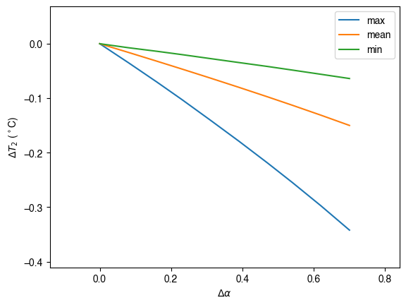
[27]:
# plot the temperature difference
ax_temp_diff = df_res_alb_T2_diff.loc[["max", "mean", "min"]].T.plot()
_ = ax_temp_diff.set_ylabel(r"$\Delta T_2$ ($^\circ$C)")
_ = ax_temp_diff.set_xlabel(r"$\Delta\alpha$")
ax_temp_diff.margins(x=0.2, y=0.2)
3.1.3.3. Background climate: air temperature#
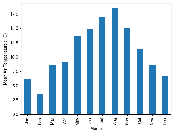
3.1.3.3.1. Examine the monthly climatology of air temperature loaded from the sample dataset#
[28]:
df_plot = df_forcing.Tair.loc["2012"].resample("1m").mean()
ax_temp = df_plot.plot.bar(color="tab:blue")
_ = ax_temp.set_xticklabels(df_plot.index.strftime("%b"))
_ = ax_temp.set_ylabel(r"Mean Air Temperature ($^\circ$C)")
_ = ax_temp.set_xlabel("Month")
3.1.3.3.2. Construct a function to perform parallel supy simulations with specified diff_airtemp_test: the difference in air temperature between the one used in simulation and loaded from sample dataset.#
Note
forcing data df_forcing has different data structure from df_state_init; so we need to modify run_supy_mgrids to implement a run_supy_mclims for different climate scenarios*
Let’s start the implementation of run_supy_mclims with a small problem of four forcing groups (i.e., climate scenarios), where the air temperatures differ from the baseline scenario with a constant bias.
[29]:
# save loaded sample datasets
df_forcing_part_test = df_forcing.loc["2012 1":"2012 7"].copy()
df_state_init_test = df_state_init.copy()
[30]:
from concurrent.futures import ThreadPoolExecutor

# create a dict with four forcing conditions as a test
n_test = 4
list_TairDiff_test = np.linspace(0.0, 2, n_test).round(2)
dict_df_forcing_x = {
    tairdiff: df_forcing_part_test.copy() for tairdiff in list_TairDiff_test
}
for tairdiff in dict_df_forcing_x:
    dict_df_forcing_x[tairdiff].loc[:, "Tair"] += tairdiff


# Helper function for parallel simulation
def run_sim_oop(key, df_forcing, df_state_init, logging_level=90):
    sim = SUEWSSimulation.from_state(df_state_init)
    sim.update_forcing(df_forcing)
    sim.run(logging_level=logging_level)
    return (key, sim.results)


# Run simulations in parallel using Python's built-in ThreadPoolExecutor
# Note: Using threads (not processes) to work in Jupyter notebooks
with ThreadPoolExecutor() as executor:
    futures = [
        executor.submit(run_sim_oop, k, df, df_state_init_test, 90)
        for k, df in dict_df_forcing_x.items()
    ]
    results = {key: result for key, result in [f.result() for f in futures]}

df_res_tairdiff_test0 = pd.concat(
    results,
    keys=list_TairDiff_test,
    names=["tairdiff"],
)
df_res_tairdiff_test = df_res_tairdiff_test0.reset_index("grid", drop=True)
[31]:
# test the performance of a parallel run
t0 = time()
# Execute the parallel simulation (already done in cell above)
t1 = time()
t_par = t1 - t0
print(f"Execution time: {t_par:.2f} s")
Execution time: 0.00 s
[32]:
# function for multi-climate `run_supy` using OOP interface and built-in parallelization
def run_supy_mclims(df_state_init, dict_df_forcing_mclims):
    from concurrent.futures import ThreadPoolExecutor

    # Helper function for parallel simulation
    def run_sim_oop(key, df_forcing, df_state_init, logging_level=90):
        sim = SUEWSSimulation.from_state(df_state_init)
        sim.update_forcing(df_forcing)
        sim.run(logging_level=logging_level)
        return (key, sim.results)

    # Run simulations in parallel using threads
    # Note: Using threads (not processes) to work in Jupyter notebooks
    with ThreadPoolExecutor() as executor:
        futures = [
            executor.submit(run_sim_oop, k, df, df_state_init, 90)
            for k, df in dict_df_forcing_mclims.items()
        ]
        results = {key: result for key, result in [f.result() for f in futures]}

    df_output_mclims0 = pd.concat(
        results,
        keys=list(dict_df_forcing_mclims.keys()),
        names=["clm"],
    )
    df_output_mclims = df_output_mclims0.reset_index("grid", drop=True)

    return df_output_mclims
3.1.3.3.3. Construct dict_df_forcing_x with multiple forcing DataFrames#
[33]:
# save loaded sample datasets
df_forcing_part_test = df_forcing.loc["2012 1":"2012 7"].copy()
df_state_init_test = df_state_init.copy()

# create a dict with a number of forcing conditions
n_test = 12  # can be set with a smaller value to save simulation time
list_TairDiff_test = np.linspace(0.0, 2, n_test).round(2)
dict_df_forcing_x = {
    tairdiff: df_forcing_part_test.copy() for tairdiff in list_TairDiff_test
}
for tairdiff in dict_df_forcing_x:
    dict_df_forcing_x[tairdiff].loc[:, "Tair"] += tairdiff
3.1.3.3.4. Perform simulations#
[34]:
# run parallel simulations using `run_supy_mclims`
t0 = time()
df_airtemp_test_x = run_supy_mclims(df_state_init_test, dict_df_forcing_x)
t1 = time()
t_par = t1 - t0
print(f"Execution time: {t_par:.2f} s")
Execution time: 72.65 s
3.1.3.3.5. Examine the results#
[35]:
df_airtemp_test = df_airtemp_test_x.SUEWS.unstack(0)
df_temp_diff = df_airtemp_test.T2.transform(lambda x: x - df_airtemp_test.T2[0.0])
df_temp_diff_ana = df_temp_diff.loc["2012 7"]
df_temp_diff_stat = df_temp_diff_ana.describe().loc[["max", "mean", "min"]].T
[36]:
ax_temp_diff_stat = df_temp_diff_stat.plot()
_ = ax_temp_diff_stat.set_ylabel(r"$\Delta T_2$ ($^\circ$C)")
_ = ax_temp_diff_stat.set_xlabel(r"$\Delta T_{a}$ ($^\circ$C)")
ax_temp_diff_stat.set_aspect("equal")
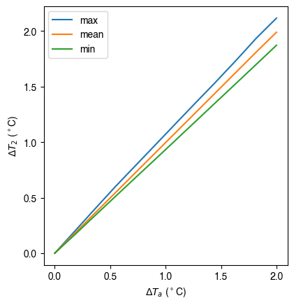
The \(T_{2}\) results indicate the increased \(T_{a}\) has different impacts on the \(T_{2}\) metrics (minimum, mean and maximum) but all increase linearly with \(T_{a}.\) The maximum \(T_{2}\) has the stronger response compared to the other metrics.