Interaction between SuPy and external models

8.1.1.1. Interaction between SuPy and external models#

8.1.1.1.1. Introduction#

SUEWS can be coupled to other models that provide or require forcing data using the SuPy single timestep running mode. We demonstrate this feature with a simple online anthropogenic heat flux model.

Anthropogenic heat flux (\(Q_F\)) is an additional term to the surface energy balance in urban areas associated with human activities (Gabey et al., 2018; Grimmond, 1992; Nie et al., 2014; 2016; Sailor, 2011). In most cities, the largest emission source is from buildings (Hamilton et al., 2009; Iamarino et al., 2011; Sailor, 2011) and is highly dependent on outdoor ambient air temperature.

8.1.1.1.1.1. load necessary packages#

[1]:

import supy as sp
import pandas as pd
import numpy as np
import matplotlib.pyplot as plt
import matplotlib.dates as mdates
import seaborn as sns

%matplotlib inline
# sp.show_version()

8.1.1.1.1.2. run SUEWS with sample data#

Note: SUEWS requires site-specific parameters; there are no generic default values. This tutorial uses sample data for demonstration.

This tutorial uses the modern SUEWSSimulation OOP interface where possible. For tight two-way model coupling (demonstrated below), low-level functions are used because single-timestep execution is not exposed in the high-level API.

8.1.1.1.1.3. Future YAML Configuration for Model Coupling#

For production workflows, YAML-based coupling configurations will provide standardised interfaces:

# Future: Modern YAML-based approach for model coupling
# coupling_config = sp.load_coupling_config("qf_coupling.yml")
# external_models = {
#     'anthropogenic_heat': QF_simple,
#     'building_energy': BuildingEnergyModel,
#     'traffic_emissions': TrafficModel
# }
# coupled_simulation = sp.run_coupled_simulation(
#     base_config="site_config.yml",
#     coupling_config=coupling_config,
#     external_models=external_models,
#     timestep_coupling=True
# )

Benefits of YAML-based coupling: - Standardised interfaces: Consistent data exchange formats - Configuration validation: Automatic checking of coupling parameters - Metadata preservation: Scientific references and model documentation - Reproducible workflows: Version-controlled coupling configurations

[ ]:

# Load sample simulation using modern OOP API
sim = sp.SUEWSSimulation.from_sample_data()

print("📊 Sample simulation loaded using modern SUEWSSimulation API")
print("✅ Ready for external model coupling")

# Extract initial state and forcing for demonstration
df_state_init = sim.df_state.copy()
df_forcing = sim.df_forcing.copy()

# turn off the snow module as unnecessary at the sample site
df_state_init.loc[:, "snowuse"] = 0

# copy for later simulations
df_state_init_def = df_state_init.copy()

# by default, two years of forcing data are included;
# to save running time for demonstration, we only use one year in this demo
df_forcing = df_forcing.loc["2012"].iloc[1:]

# set QF as zero for later comparison
df_forcing_def = df_forcing.copy()
grid = df_state_init_def.index[0]
df_state_init_def.loc[:, "emissionsmethod"] = 0
df_forcing_def["qf"] = 0

# run simulation using modern API
sim_def = sp.SUEWSSimulation(df_forcing=df_forcing_def, df_state=df_state_init_def)
df_output_def = sim_def.run().df_output.loc[grid, "SUEWS"]

8.1.1.1.2. a simple QF model: `QF_simple`#

8.1.1.1.2.1. model description#

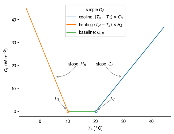
For demonstration purposes we have created a very simple model instead of using the SUEWS \(Q_F\) (Järvi et al. 2011) with feedback from outdoor air temperature. The simple \(Q_F\) model considers only building heating and cooling:

\[\begin{split}Q_F=\left\{ \begin{array}{ll} (T_2-T_C)\times C_B,\;T_2 > T_C\\ (T_H-T_2)\times H_B,\;T_2 < T_H\\ Q_{F0} \end{array} \right.\end{split}\]

where \(T_C\) (\(T_H\)) is the cooling (heating) threshold temperature of buildings, \(𝐶_B\) (\(𝐻_B\)) is the building cooling (heating) rate, and \(𝑄_{F0}\) is the baseline anthropogenic heat. The parameters used are: \(𝑇_C\) (\(𝑇_H\)) set as 20 °C (10 °C), \(𝐶_B\) (\(𝐻_B\)) set as 1.5 \(\mathrm{W\ m^{-2}\ K^{-1}}\) (3 \(\mathrm{W\ m^{-2}\ K^{-1}}\)) and \(Q_{F0}\) is set as 0 \(\mathrm{W\ m^{-2}}\), implying other building activities (e.g. lighting, water heating, computers) are zero and therefore do not change the temperature or change with temperature.

8.1.1.1.2.2. implementation#

[3]:

def QF_simple(T2):
    qf_cooling = (T2 - 20) * 5 if T2 > 20 else 0
    qf_heating = (10 - T2) * 10 if T2 < 10 else 0
    qf_res = np.max([qf_heating, qf_cooling]) * 0.3
    return qf_res

Visualise the QF_simple model:

[ ]:

ser_temp = pd.Series(np.arange(-5, 45, 0.5), index=np.arange(-5, 45, 0.5)).rename(
    "temp_C"
)
ser_qf_heating = (
    ser_temp.loc[-5:10].map(QF_simple).rename(r"heating:$(T_H-T_a) \times H_B$")
)
ser_qf_cooling = (
    ser_temp.loc[20:45].map(QF_simple).rename(r"cooling: $(T_a-T_C) \times C_B$")
)
ser_qf_zero = ser_temp.loc[10:20].map(QF_simple).rename("baseline: $Q_{F0}$")
df_temp_qf = pd.concat(
    [ser_temp, ser_qf_cooling, ser_qf_heating, ser_qf_zero], axis=1
).set_index("temp_C")
ax_qf_func = df_temp_qf.plot()
_ = ax_qf_func.set_xlabel("$T_2$ ($^\circ$C)")
_ = ax_qf_func.set_ylabel("$Q_F$ ($ \mathrm{W \ m^{-2}}$)")
_ = ax_qf_func.legend(title="simple $Q_F$")
_ = ax_qf_func.annotate(
    "$T_C$",
    xy=(20, 0),
    xycoords="data",
    xytext=(25, 5),
    textcoords="data",
    arrowprops=dict(
        arrowstyle="->",
        color="0.5",
        shrinkA=5,
        shrinkB=5,
        patchA=None,
        patchB=None,
        connectionstyle="arc3",
    ),
)

_ = ax_qf_func.annotate(
    "$T_H$",
    xy=(10, 0),
    xycoords="data",
    xytext=(5, 5),
    textcoords="data",
    arrowprops=dict(
        arrowstyle="->",
        color="0.5",
        shrinkA=5,
        shrinkB=5,
        patchA=None,
        patchB=None,
        connectionstyle="arc3",
    ),
)
_ = ax_qf_func.annotate(
    "slope: $C_B$",
    xy=(30, QF_simple(30)),
    xycoords="data",
    xytext=(20, 20),
    textcoords="data",
    arrowprops=dict(
        arrowstyle="->",
        color="0.5",
        shrinkA=5,
        shrinkB=5,
        patchA=None,
        patchB=None,
        connectionstyle="arc3, rad=0.3",
    ),
)
_ = ax_qf_func.annotate(
    "slope: $H_B$",
    xy=(5, QF_simple(5)),
    xycoords="data",
    xytext=(10, 20),
    textcoords="data",
    arrowprops=dict(
        arrowstyle="->",
        color="0.5",
        shrinkA=5,
        shrinkB=5,
        patchA=None,
        patchB=None,
        connectionstyle="arc3, rad=-0.3",
    ),
)
_ = ax_qf_func.plot(10, 0, "o", color="C1", fillstyle="none")
_ = ax_qf_func.plot(20, 0, "o", color="C0", fillstyle="none")

../_images/integration_external-interaction_16_0.png

8.1.1.1.3. communication between `supy` and `QF_simple`#

8.1.1.1.3.1. construct a new coupled function#

Note: The coupling function below uses low-level functions because tight two-way coupling requires single-timestep execution, which is not exposed in the high-level SUEWSSimulation API. For production coupling workflows, future YAML-based coupling configurations (shown above) will provide standardised interfaces.

The coupling between the simple \(Q_F\) model and SuPy is done via the low-level function suews_cal_tstep, which is an interface function in charge of communications between SuPy frontend and the calculation kernel. By setting SuPy to receive external \(Q_F\) as forcing, at each timestep, the simple \(Q_F\) model is driven by the SuPy output \(T_2\) and provides SuPy with \(Q_F\), which thus forms a two-way coupled loop.

[11]:

# load extra low-level functions from supy to construct interactive functions
from supy._post import pack_df_output_line, pack_df_state
from supy._run import suews_cal_tstep, pack_grid_dict
import numpy as np


def run_supy_qf(df_forcing_test, df_state_init_test):
    grid = df_state_init_test.index[0]
    df_state_init_test.loc[grid, "emissionsmethod"] = 0

    df_forcing_test = df_forcing_test.assign(
        metforcingdata_grid=0,
        ts5mindata_ir=0,
    ).rename(
        # remanae is a workaround to resolve naming inconsistency between
        # suews fortran code interface and input forcing file headers
        columns={
            "%" + "iy": "iy",
            "id": "id",
            "it": "it",
            "imin": "imin",
            "qn": "qn1_obs",
            "qh": "qh_obs",
            "qe": "qe",
            "qs": "qs_obs",
            "qf": "qf_obs",
            "U": "avu1",
            "RH": "avrh",
            "Tair": "temp_c",
            "pres": "press_hpa",
            "rain": "precip",
            "kdown": "avkdn",
            "snow": "snowfrac_obs",
            "ldown": "ldown_obs",
            "fcld": "fcld_obs",
            "Wuh": "wu_m3",
            "xsmd": "xsmd",
            "lai": "lai_obs",
            "kdiff": "kdiff",
            "kdir": "kdir",
            "wdir": "wdir",
        }
    )

    t2_ext = df_forcing_test.iloc[0].temp_c
    qf_ext = QF_simple(t2_ext)

    # initialise dicts for holding results
    dict_state = {}
    dict_output = {}

    # starting tstep
    t_start = df_forcing_test.index[0]
    # convert df to dict with `itertuples` for better performance
    dict_forcing = {row.Index: row._asdict() for row in df_forcing_test.itertuples()}
    # dict_state is used to save model states for later use
    dict_state = {
        (t_start, grid): pack_grid_dict(series_state_init)
        for grid, series_state_init in df_state_init_test.iterrows()
    }

    # just use a single grid run for the test coupling
    for tstep in df_forcing_test.index:
        # load met forcing at `tstep`
        met_forcing_tstep = dict_forcing[tstep]
        # inject `qf_ext` to `met_forcing_tstep`
        met_forcing_tstep["qf_obs"] = qf_ext

        # Add missing variables expected by suews_cal_tstep
        # These are needed for compatibility with the current SUEWS interface
        met_forcing_tstep["len_sim"] = np.array(1, dtype=int)  # Single timestep
        met_forcing_tstep["metforcingblock"] = np.array([[0]], order="F")  # Placeholder
        met_forcing_tstep["flag_test"] = False  # Not in debug mode

        # update model state
        dict_state_start = dict_state[(tstep, grid)]

        dict_state_end, dict_output_tstep = suews_cal_tstep(
            dict_state_start, met_forcing_tstep
        )
        # the fourth to the last is `T2` stored in the result array
        t2_ext = dict_output_tstep["dataoutlinesuews"][-4]
        qf_ext = QF_simple(t2_ext)

        dict_output.update({(tstep, grid): dict_output_tstep})
        dict_state.update({(tstep + tstep.freq, grid): dict_state_end})

    # pack results as easier DataFrames
    df_output_test = pack_df_output_line(dict_output).swaplevel(0, 1)
    df_state_test = pack_df_state(dict_state).swaplevel(0, 1)
    return df_output_test.loc[grid, "SUEWS"], df_state_test

8.1.1.1.3.2. simulations for summer and winter months#

The simulation using SuPy coupled is performed for London 2012. The data analysed are a summer (July) and a winter (December) month. Initially \(Q_F\) is 0 \(\mathrm{W\ m^{-2}}\) the \(T_2\) is determined and used to determine \(Q_{F[1]}\) which in turn modifies \(T_{2[1]}\) and therefore modifies \(Q_{F[2]}\) and the diagnosed \(T_{2[2]}\).

8.1.1.1.3.2.1. spin-up run (January to June) for summer simulation#

[ ]:

# spin-up run using modern OOP API
sim_june = sp.SUEWSSimulation(df_forcing=df_forcing.loc[:"2012 6"], df_state=df_state_init)
sim_june.run()
df_output_june = sim_june.df_output
df_state_jul = sim_june.df_state

8.1.1.1.3.2.2. spin-up run (July to October) for winter simulation#

[ ]:

# spin-up run using modern OOP API
sim_oct = sp.SUEWSSimulation(df_forcing=df_forcing.loc["2012 7":"2012 11"], df_state=df_state_jul)
sim_oct.run()
df_output_oct = sim_oct.df_output
df_state_dec = sim_oct.df_state

8.1.1.1.3.2.3. coupled simulation#

[16]:

# df_output_test_summer, df_state_summer_test = run_supy_qf(
#     df_forcing.loc["2012-07"], df_state_jul.copy()
# )
# df_output_test_winter, df_state_winter_test = run_supy_qf(
#     df_forcing.loc["2012-12"], df_state_dec.copy()
# )

8.1.1.1.3.3. examine the results#

8.1.1.1.3.3.1. sumer#

[17]:

# var = "QF"
# var_label = "$Q_F$ ($ \mathrm{W \ m^{-2}}$)"
# var_label_right = "$\Delta Q_F$ ($ \mathrm{W \ m^{-2}}$)"
# period = "2012-07"
# df_test = df_output_test_summer
# y1 = df_test.loc[period, var].rename("qf_simple")
# y2 = df_output_def.loc[period, var].rename("suews")
# y3 = (y1 - y2).rename("diff")
# df_plot = pd.concat([y1, y2, y3], axis=1)
# ax = df_plot.plot(secondary_y="diff")
# _ = ax.set_ylabel(var_label)
# _ = ax.right_ax.set_ylabel(var_label_right)
# lines = ax.get_lines() + ax.right_ax.get_lines()
# _ = ax.legend(lines, [l.get_label() for l in lines], loc="best")

[18]:

# var = "T2"
# var_label = "$T_2$ ($^{\circ}$C)"
# var_label_right = "$\Delta T_2$ ($^{\circ}$C)"
# period = "2012-07"
# df_test = df_output_test_summer
# y1 = df_test.loc[period, var].rename("qf_simple")
# y2 = df_output_def.loc[period, var].rename("suews")
# y3 = (y1 - y2).rename("diff")
# df_plot = pd.concat([y1, y2, y3], axis=1)
# ax = df_plot.plot(secondary_y="diff")
# _ = ax.set_ylabel(var_label)
# _ = ax.right_ax.set_ylabel(var_label_right)
# lines = ax.get_lines() + ax.right_ax.get_lines()
# _ = ax.legend(lines, [l.get_label() for l in lines], loc="best")

8.1.1.1.3.3.2. winter#

[19]:

# var = "QF"
# var_label = "$Q_F$ ($ \mathrm{W \ m^{-2}}$)"
# var_label_right = "$\Delta Q_F$ ($ \mathrm{W \ m^{-2}}$)"
# period = "2012 12"
# df_test = df_output_test_winter
# y1 = df_test.loc[period, var].rename("qf_simple")
# y2 = df_output_def.loc[period, var].rename("suews")
# y3 = (y1 - y2).rename("diff")
# df_plot = pd.concat([y1, y2, y3], axis=1)
# ax = df_plot.plot(secondary_y="diff")
# _ = ax.set_ylabel(var_label)
# _ = ax.right_ax.set_ylabel(var_label_right)
# lines = ax.get_lines() + ax.right_ax.get_lines()
# _ = ax.legend(lines, [l.get_label() for l in lines], loc="best")

[20]:

# var = "T2"
# var_label = "$T_2$ ($^{\circ}$C)"
# var_label_right = "$\Delta T_2$ ($^{\circ}$C)"
# period = "2012 12"
# df_test = df_output_test_winter
# y1 = df_test.loc[period, var].rename("qf_simple")
# y2 = df_output_def.loc[period, var].rename("suews")
# y3 = (y1 - y2).rename("diff")
# df_plot = pd.concat([y1, y2, y3], axis=1)
# ax = df_plot.plot(secondary_y="diff")
# _ = ax.set_ylabel(var_label)
# _ = ax.right_ax.set_ylabel(var_label_right)
# lines = ax.get_lines() + ax.right_ax.get_lines()
# _ = ax.legend(lines, [l.get_label() for l in lines], loc="center right")

8.1.1.1.3.3.3. comparison in \(\Delta Q_F\)-\(\Delta T2\) feedback between summer and winter#

[21]:

# # filter results using `where` to choose periods when `QF_simple` is effective
# # (i.e. activated by outdoor air temperatures)
# df_diff_summer = (
#     (df_output_test_summer - df_output_def)
#     .where(df_output_def.T2 > 20, np.nan)
#     .dropna(how="all", axis=0)
# )
# df_diff_winter = (
#     (df_output_test_winter - df_output_def)
#     .where(df_output_test_winter.T2 < 10, np.nan)
#     .dropna(how="all", axis=0)
#     .loc["20121215":]
# )


# df_diff_season = pd.concat(
#     [
#         df_diff_winter.assign(season="winter"),
#         df_diff_summer.assign(season="summer"),
#     ]
# ).loc[:, ["season", "QF", "T2"]]
# g = sns.lmplot(
#     data=df_diff_season,
#     x="QF",
#     y="T2",
#     hue="season",
#     height=4,
#     truncate=False,
#     markers="o",
#     legend_out=False,
#     scatter_kws={
#         "s": 1,
#         "zorder": 0,
#         "alpha": 0.8,
#     },
#     line_kws={"zorder": 6, "linestyle": "--"},
# )
# _ = g.set_axis_labels(
#     "$\Delta Q_F$ ($ \mathrm{W \ m^{-2}}$)",
#     "$\Delta T_2$ ($^{\circ}$C)",
# )
# _ = g.ax.legend(markerscale=4)
# _ = g.despine(top=False, right=False)

The above figure indicates a positive feedback, as \(Q_F\) is increased there is an elevated \(T_2\) but with different magnitudes given the non-linearlity in the SUEWS modelling system. Of particular note is the positive feedback loop under warm air temperatures: the anthropogenic heat emissions increase which in turn elevates the outdoor air temperature causing yet more anthropogenic heat release. Note that London is relatively cool so the enhancement is much less than it would be in warmer cities.