Tip

1. Need help? Please let us know in the SUEWS Community.

2. Please report issues with the manual on GitHub Issues (or use Report Issue for This Page for page-specific feedback).

3. Please cite SUEWS with proper information from our Zenodo page.

3.1. SUEWS Quick Start Tutorial

Essential SUEWS workflow using the modern SuPy (Python) interface.

This tutorial demonstrates the complete workflow for running urban climate simulations with SUEWS:

1. Load sample data

2. Run simulation

3. Explore results (statistics, plotting, resampling)

What is SUEWS?

SUEWS (Surface Urban Energy and Water Balance Scheme) is an urban climate model that simulates energy and water fluxes in urban environments. SuPy is the modern Python interface that provides powerful data analysis capabilities and seamless integration with the scientific Python ecosystem.

import matplotlib.pyplot as plt
import pandas as pd

from supy import SUEWSSimulation

3.1.1. Load Sample Data

SuPy includes built-in sample data to get you started immediately. Load sample data for the simulation using the modern OOP API.

sim = SUEWSSimulation.from_sample_data()

print("Sample data loaded successfully!")
print(f"Grid ID: {sim.state_init.index[0]}")
print(f"Forcing period: {sim.forcing.time_range}")
print(f"Time steps: {len(sim.forcing)}")

Sample data loaded successfully!
Grid ID: 1
Forcing period: (Timestamp('2012-01-01 00:05:00'), Timestamp('2013-01-01 00:00:00'))
Time steps: 105408

3.1.2. Understanding Input Data

SUEWS requires two main input datasets:

• state_init: Initial conditions and site configuration

• forcing: Meteorological forcing data (time series)

Access these through the simulation object’s properties.

# Surface characteristics: building and tree heights
print("Building and tree heights:")
print(sim.state_init.loc[:, ["bldgh", "evetreeh", "dectreeh"]])

# Surface fractions by land cover type
print("\nSurface fractions:")
print(sim.state_init.filter(like="sfr_surf"))

Building and tree heights:
var     bldgh evetreeh dectreeh
ind_dim     0        0        0
grid
1        22.0     13.1     13.1

Surface fractions:
var     sfr_surf
ind_dim     (0,)  (1,) (2,)  (3,)  (4,) (5,)  (6,)
grid
1           0.43  0.38  0.0  0.02  0.03  0.0  0.14

3.1.3. Visualise Forcing Data

The forcing data drives the simulation. Access forcing variables directly as attributes of sim.forcing.

# Access forcing variables through the OOP interface
print("\nForcing data summary:")
print(f"  Air temperature range: {sim.forcing.Tair.min():.1f} to {sim.forcing.Tair.max():.1f} C")
print(f"  Wind speed range: {sim.forcing.U.min():.1f} to {sim.forcing.U.max():.1f} m/s")
print(f"  Total rainfall: {sim.forcing.rain.sum():.1f} mm")

# Slice forcing data by time (returns new SUEWSForcing object).
# Drop the first row with `.iloc[1:]` because accumulated variables
# (e.g. rainfall) for the partial period at the slice boundary are
# incomplete, making that row invalid as forcing input.
forcing_sliced = sim.forcing["2012-01":"2012-03"].iloc[1:]

# Update simulation with the time-sliced forcing
sim.update_forcing(forcing_sliced)

# Plot key meteorological variables
list_var_forcing = ["kdown", "Tair", "RH", "pres", "U", "rain"]
dict_var_label = {
    "kdown": r"Incoming Solar Radiation ($\mathrm{W\ m^{-2}}$)",
    "Tair": r"Air Temperature ($^\circ$C)",
    "RH": "Relative Humidity (%)",
    "pres": "Air Pressure (hPa)",
    "rain": "Rainfall (mm)",
    "U": r"Wind Speed ($\mathrm{m\ s^{-1}}$)",
}

Forcing data summary:
  Air temperature range: -5.7 to 28.8 C
  Wind speed range: 0.2 to 11.2 m/s
  Total rainfall: 821.0 mm

Tip

When resampling forcing data, call resample() first, then select columns. SUEWSForcing.resample() applies the correct aggregation method for each variable type (rain=sum, radiation=mean, instantaneous=last). Selecting columns first bypasses this logic.

# Resample to hourly for cleaner plots
df_plot_forcing = forcing_sliced.resample("1h")[list_var_forcing]

fig, axes = plt.subplots(6, 1, figsize=(10, 12), sharex=True)
for ax, var in zip(axes, list_var_forcing):
    df_plot_forcing[var].plot(ax=ax, legend=False)
    ax.set_ylabel(dict_var_label[var])
fig.tight_layout()

3.1.4. Modify Input Parameters

Modify surface parameters using the update_config method. This is the recommended approach for parameter changes.

# View original surface fractions
print("Original surface fractions:")
print(sim.state_init.loc[:, "sfr_surf"])

# Modify surface fractions using update_config
sim.update_config({"initial_states": {"sfr_surf": [0.1, 0.1, 0.2, 0.3, 0.25, 0.05, 0]}})

print("\nModified surface fractions:")
print(sim.state_init.loc[:, "sfr_surf"])

Original surface fractions:
ind_dim  (0,)  (1,)  (2,)  (3,)  (4,)  (5,)  (6,)
grid
1        0.43  0.38   0.0  0.02  0.03   0.0  0.14

Modified surface fractions:
ind_dim  (0,)  (1,)  (2,)  (3,)  (4,)  (5,)  (6,)
grid
1        0.43  0.38   0.0  0.02  0.03   0.0  0.14

3.1.5. Run Simulation

With forcing data and initial conditions ready, run the SUEWS simulation. The run() method returns a SUEWSOutput object for convenient access.

output = sim.run()

print(f"Simulation complete: {len(output.times)} timesteps")
print(f"Output groups: {output.groups}")
print(f"Grids: {output.grids}")

Simulation complete: 26206 timesteps
Output groups: ['BEERS', 'DailyState', 'debug', 'EHC', 'NHood', 'RSL', 'snow', 'SPARTACUS', 'STEBBS', 'SUEWS']
Grids: [1]

3.1.6. Explore Results: Statistics

Access output variables directly as attributes of the output object. Use pandas’ built-in methods for quick statistical summaries.

# Access energy balance variables via SUEWS output group
df_suews = output.SUEWS

print("Energy balance statistics:")
print(f"  Net radiation (QN): mean = {df_suews['QN'].mean():.1f} W/m2")
print(f"  Sensible heat (QH): mean = {df_suews['QH'].mean():.1f} W/m2")
print(f"  Latent heat (QE): mean = {df_suews['QE'].mean():.1f} W/m2")
print(f"  Storage heat (QS): mean = {df_suews['QS'].mean():.1f} W/m2")

# Detailed statistics
df_suews.loc[:, ["QN", "QS", "QH", "QE", "QF"]].describe()

Energy balance statistics:
  Net radiation (QN): mean = 10.8 W/m2
  Sensible heat (QH): mean = 70.3 W/m2
  Latent heat (QE): mean = 16.1 W/m2
  Storage heat (QS): mean = 16.2 W/m2

var	QN	QS	QH	QE	QF
count	26206.000000	26206.000000	26206.000000	26206.000000	26206.000000
mean	10.812930	16.161789	70.264978	16.056442	91.670278
std	108.169202	73.468485	54.640931	13.603767	35.134039
min	-84.461392	-83.898514	-42.295955	2.128621	32.930049
25%	-48.146256	-21.913831	25.612437	7.769746	58.325762
50%	-36.461484	-13.508590	56.375046	12.418750	95.320954
75%	20.068137	23.287372	105.498358	19.386790	122.766324
max	510.527926	369.617174	287.090099	139.340060	161.500795

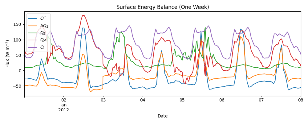
3.1.7. Explore Results: Weekly Energy Balance

Plot the surface energy balance for one week to see diurnal patterns.

dict_var_disp = {
    "QN": r"$Q^*$",
    "QS": r"$\Delta Q_S$",
    "QE": "$Q_E$",
    "QH": "$Q_H$",
    "QF": "$Q_F$",
}

# Get grid ID for indexing
grid = output.grids[0]

# Select first week of available data for plotting
start_date = output.times[0]
end_date = start_date + pd.Timedelta(days=7)

fig, ax = plt.subplots(figsize=(10, 4))
(
    df_suews.loc[grid]
    .loc[start_date:end_date, ["QN", "QS", "QE", "QH", "QF"]]
    .rename(columns=dict_var_disp)
    .plot(ax=ax)
)
ax.set_xlabel("Date")
ax.set_ylabel(r"Flux ($\mathrm{W\ m^{-2}}$)")
ax.set_title("Surface Energy Balance (One Week)")
ax.legend()
plt.tight_layout()

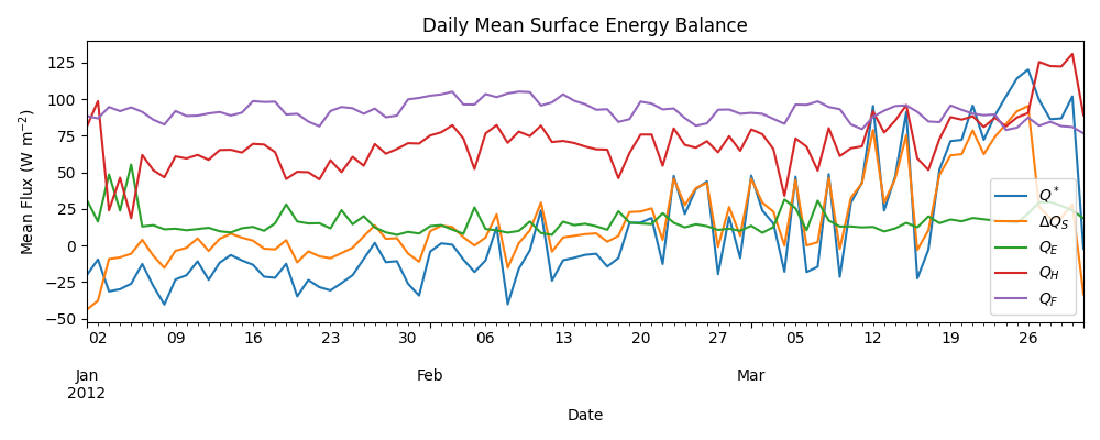
3.1.8. Temporal Resampling: Daily Patterns

SUEWS runs at 5-minute intervals. Resampling to daily values reveals seasonal patterns.

rsmp_1d = df_suews.loc[grid].resample("1d")
df_1d_mean = rsmp_1d.mean()
df_1d_sum = rsmp_1d.sum()

# Plot daily mean energy balance
fig, ax = plt.subplots(figsize=(10, 4))
(
    df_1d_mean.loc[:, ["QN", "QS", "QE", "QH", "QF"]]
    .rename(columns=dict_var_disp)
    .plot(ax=ax)
)
ax.set_xlabel("Date")
ax.set_ylabel(r"Mean Flux ($\mathrm{W\ m^{-2}}$)")
ax.set_title("Daily Mean Surface Energy Balance")
ax.legend()
plt.tight_layout()

/private/tmp/claude/-Users-tingsun-conductor-workspaces-suews-havana-v1/41d4ccd2-265e-4416-b3db-fa0bcb209699/scratchpad/docs-worktree/docs/source/tutorials/tutorial_01_quick_start.py:202: Pandas4Warning: 'd' is deprecated and will be removed in a future version, please use 'D' instead.
  rsmp_1d = df_suews.loc[grid].resample("1d")

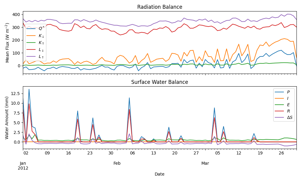
3.1.9. Radiation and Water Balance

Examine radiation components and water balance using daily aggregates.

dict_var_disp_full = {
    "QN": r"$Q^*$",
    "Kdown": r"$K_{\downarrow}$",
    "Kup": r"$K_{\uparrow}$",
    "Ldown": r"$L_{\downarrow}$",
    "Lup": r"$L_{\uparrow}$",
    "Rain": "$P$",
    "Irr": "$I$",
    "Evap": "$E$",
    "RO": "$R$",
    "TotCh": r"$\Delta S$",
}

fig, axes = plt.subplots(2, 1, figsize=(10, 6), sharex=True)

# Radiation balance
(
    df_1d_mean.loc[:, ["QN", "Kdown", "Kup", "Ldown", "Lup"]]
    .rename(columns=dict_var_disp_full)
    .plot(ax=axes[0])
)
axes[0].set_ylabel(r"Mean Flux ($\mathrm{W\ m^{-2}}$)")
axes[0].set_title("Radiation Balance")
axes[0].legend()

# Water balance
(
    df_1d_sum.loc[:, ["Rain", "Irr", "Evap", "RO", "TotCh"]]
    .rename(columns=dict_var_disp_full)
    .plot(ax=axes[1])
)
axes[1].set_xlabel("Date")
axes[1].set_ylabel("Water Amount (mm)")
axes[1].set_title("Surface Water Balance")
axes[1].legend()

plt.tight_layout()

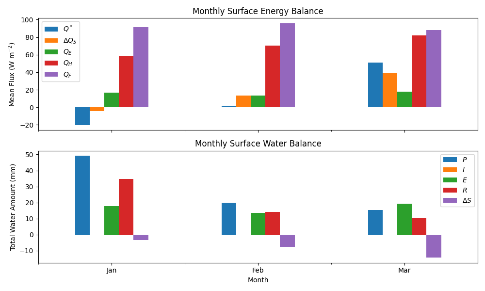
3.1.10. Monthly Patterns

Aggregate to monthly values for seasonal overview using bar charts.

df_plot = df_suews.loc[grid].copy()
df_plot.index = df_plot.index.set_names("Month")
rsmp_1M = df_plot.shift(-1).dropna(how="all").resample("1ME")
df_1M_mean = rsmp_1M.mean()
df_1M_sum = rsmp_1M.sum()
# Convert index to period for better month display
df_1M_mean.index = df_1M_mean.index.to_period("M")
df_1M_sum.index = df_1M_sum.index.to_period("M")

# Month names for labels
name_mon = [x.strftime("%b") for x in rsmp_1M.groups]

fig, axes = plt.subplots(2, 1, sharex=True, figsize=(10, 6))

# Monthly energy balance
(
    df_1M_mean.loc[:, ["QN", "QS", "QE", "QH", "QF"]]
    .rename(columns=dict_var_disp)
    .plot(ax=axes[0], kind="bar")
)
axes[0].set_ylabel(r"Mean Flux ($\mathrm{W\ m^{-2}}$)")
axes[0].set_title("Monthly Surface Energy Balance")
axes[0].legend()

# Monthly water balance
(
    df_1M_sum.loc[:, ["Rain", "Irr", "Evap", "RO", "TotCh"]]
    .rename(columns=dict_var_disp_full)
    .plot(ax=axes[1], kind="bar")
)
axes[1].set_xlabel("Month")
axes[1].set_ylabel("Total Water Amount (mm)")
axes[1].set_title("Monthly Surface Water Balance")
axes[1].xaxis.set_ticklabels(name_mon, rotation=0)
axes[1].legend()

plt.tight_layout()

3.1.11. Summary

This tutorial demonstrated the essential SUEWS workflow:

1. Load sample data using from_sample_data()

2. Run simulation with run() which returns SUEWSOutput

3. Explore results using the OOP interface for intuitive variable access

Key concepts covered:

• Energy balance components: Q*, QH, QE, QS, QF

• Radiation balance: Kdown, Kup, Ldown, Lup

• Water balance: Rain, Evap, Runoff, Storage change

• Temporal resampling: 5-min to hourly, daily, monthly

Next steps:

• Set Up SUEWS for Your Own Site - Configure SUEWS for your own site

• tutorial_03_impact_studies - Sensitivity analysis and scenario modelling