

Tip
Need help? Please let us know in the SUEWS Community.
Please report issues with the manual on GitHub Issues (or use Report Issue for This Page for page-specific feedback).
Please cite SUEWS with proper information from our Zenodo page.
Warning
DEPRECATED: This table-based input format is deprecated as of 2025. Please use the modern YAML format instead. See our transition guide for migration help.
SUEWS_OHMCoefficients.txt#
OHM, the Objective Hysteresis Model [Grimmond et al., 1991] calculates the storage heat flux as a function of net all-wave radiation and surface characteristics.
For each surface, OHM requires three model coefficients (a1, a2, a3). The three should be selected as a set.
The SUEWS_OHMCoefficients.txt file provides these coefficients for each surface type.
A variety of values has been derived for different materials and can be found in the literature (see: Typical Values).
SUEWS blends the four coefficient sets according to surface wetness and season, rather than switching abruptly between them. The configured summer/winter and wet/dry thresholds are the centres of transition zones.
To use the same coefficients irrespective of wet/dry and summer/winter conditions, use the same code for all four OHM columns (
OHMCode_SummerWet,OHMCode_SummerDry,OHMCode_WinterWetandOHMCode_WinterDry).
Smooth coefficient transitions
For each of the three OHM coefficients, SUEWS calculates a summer weight
w_s and a wet weight w_w. It then combines the summer-wet (SW),
summer-dry (SD), winter-wet (WW) and winter-dry (WD) coefficient sets:
where c represents a1, a2 or a3. The weights are clamped to
the interval from 0 to 1, so the original coefficient sets are recovered
outside the transition zones.
The transition bands are deliberately narrow. They exist to remove the discontinuity at each threshold, where an arbitrarily small change in temperature or wetness previously switched the whole coefficient set; they are not intended to re-blend the coefficients over a wide physical range. Outside the bands the model reproduces the unblended coefficients exactly.
Summer/winter transition:
w_suses the 5-day running mean air temperature. The configuredOHMThresh_SWvalue is the centre of a 0.5 degC-wide transition. Winter coefficients have full weight at and belowOHMThresh_SW - 0.25 degC; summer coefficients have full weight at and aboveOHMThresh_SW + 0.25 degC.Surface-wetness transition: the calculated surface water store gives zero wet weight at 0 mm, increases linearly between 0 and 0.1 mm, and gives full wet weight at and above 0.1 mm. This rule applies to all non-snow surfaces. It is the only wet/dry route for paved and building surfaces, which have no soil store.
Soil-moisture transition: for evergreen trees, deciduous trees, grass and bare soil with positive soil-store capacity, the soil-moisture ratio also contributes a wet weight.
OHMThresh_WDis the centre of a 0.04-wide transition: full dry weight occurs at and belowOHMThresh_WD - 0.02and full wet weight at and aboveOHMThresh_WD + 0.02.Combined wetness: SUEWS uses the larger of the surface-wetness and soil-moisture wet weights. A wet surface store therefore retains wet coefficients even when the underlying soil is dry.
Snow exception: snow storage heat continues to use the winter-wet coefficient set directly and is not included in this blending calculation.
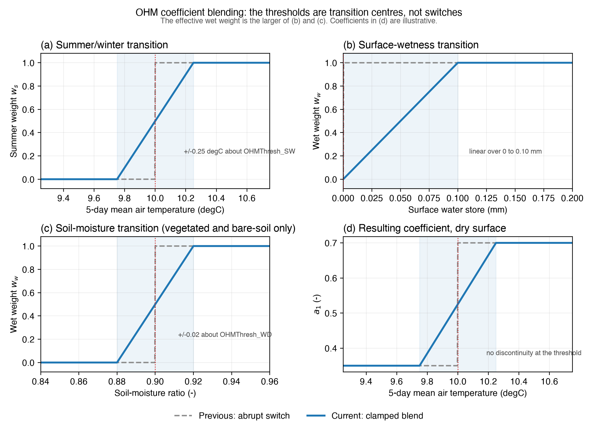
Blending of the OHM coefficient sets. Panels (a) to (c) show the summer
weight w_s and the wet weight w_w as functions of the 5-day mean air
temperature, the surface water store and the soil-moisture ratio. The
configured thresholds (OHMThresh_SW, OHMThresh_WD) are the centres of
the shaded transition zones rather than switching points, and the weights are
clamped to 0 and 1 so the original coefficient sets are recovered outside
those zones. Panel (d) shows the consequence for a1 on a dry surface:
the coefficient now varies continuously across the seasonal threshold instead
of jumping. Generated by docs/plot_ohm_transitions.py.#
Note
AnOHM (set in RunControl.nml by
StorageHeatMethod= 3) does not use the coefficients specified in SUEWS_OHMCoefficients.txt but instead requires three parameters to be specified for each surface type (including snow): heat capacity (AnOHM_Cp), thermal conductivity (AnOHM_Kk) and bulk transfer coefficient (AnOHM_Ch). These are specified in SUEWS_NonVeg.txt, SUEWS_Veg.txt, SUEWS_Water.txt and SUEWS_Snow.txt. No additional files are required for AnOHM.AnOHM is under development in v2018b and should NOT be used!
No. |
Column Name |
Use |
Description |
|---|---|---|---|
1 |
Code linking to a corresponding look-up table. |
||
2 |
Coefficient for Q* term [-] |
||
3 |
Coefficient for |
||
4 |
Constant term [W m-2] |
An example SUEWS_OHMCoefficients.txt can be found below:
1 2 3 4
Code a1 a2 a3 ! Surface type Reference Not recommended (NR)
10 0.71 0.04 -39.7 ! "Canyon (E-W), Japan" Yosheida (1990/91)
11 0.32 0.01 -27.7 ! "Canyon, Vancouver" Nunez (1974)
100 0.515 0.025 -33.7 ! Canyon (average)
200 0.336 0.313 -31.4 ! "Vegetation (average). This is the average of Codes 20, 30, 50, 51, 52, 53, 60 (i.e. includes soil and water)."
201 0.215 0.325 -19.85 ! NEW Vegetation only (average of codes 20 and 30).
2011 0.230 0.276 -16.91 ! Code 201 x Mulitplier for summer
2012 0.270 -0.435 6.62 ! Code 201 x Multiplier for winter
20 0.11 0.11 -12.3 ! Mixed Forest McCaughey (1985)
30 0.32 0.54 -27.4 ! Short grass Doll et al. (1985)
50 0.38 0.56 -27.3 ! Bare soil Novak (1982)
51 0.33 0.07 -34.9 ! Bare soil (wet) Fuchs & Hadas (1972)
52 0.35 0.43 -36.5 ! Bare soil (dry) Fuchs & Hadas (1972)
53 0.36 0.27 -42.4 ! Bare soil Asaeda & Ca (1983)
55 0.355 0.335 -35.275 ! "Bare soil (average). This is the average of Codes 50, 51, 52, 53."
551 0.379 0.284 -30.05 ! Code 55 x Mulitplier for summer
552 0.445 -0.448 11.77 ! Code 55 x Mulitplier for winter
60 0.5 0.21 -39.1 ! Water (shallow - turbid) Souch et al. (1998)
601 0.534 0.178 -33.31 ! Code 60 x Multiplier for summer
602 0.627 -0.281 13.05 ! Code 60 x Multiplier for winter
61 0.25 0.6 -30 ! Snow Jarvi et al. (2014)
713 0.17 0.1 -17 ! "Roof (tar and gravel, summer)" summer
701 0.3 0.96 -24 ! "Roof (commerical or industrial, gravel, dry, WS < 1 m/s, Vancouver)" "Meyn & Oke (2009) Table 4, Pg 750"
702 0.26 0.89 -21 ! "Roof (commerical or industrial, gravel, dry, WS 1-1.4 m/s, Vancouver)" "Meyn & Oke (2009) Table 4, Pg 750"
703 0.23 0.87 -24 ! "Roof (commerical or industrial, gravel, dry, WS 1.5-2 m/s, Vancouver)" "Meyn & Oke (2009) Table 4, Pg 750"
704 0.23 0.69 -21 ! "Roof (commerical or industrial, gravel, wet, WS 0.9-1.9 m/s, Vancouver)" "Meyn & Oke (2009) Table 4, Pg 750"
705 0.06 0.28 -3 ! "Roof (commerical or industrial, bitumen spread over flat industrial membrane, wet & dry, WS 1.1-2 m/s, Vancouver)" "Meyn & Oke (2009) Table 4, Pg 750"
706 0.15 0.28 -6 ! "Roof (residential, asphalt shingle on plywood, dry, WS < 1 m/s, Vancouver)" "Meyn & Oke (2009) Table 4, Pg 750"
707 0.12 0.25 -5 ! "Roof (residential, asphalt shingle on plywood, dry, WS < 1.0-1.4 m/s, Vancouver)" "Meyn & Oke (2009) Table 4, Pg 750"
708 0.1 0.23 -6 ! "Roof (residential, asphalt shingle on plywood, dry, WS < 2 m/s, Vancouver)" "Meyn & Oke (2009) Table 4, Pg 750"
709 0.09 0.18 -1 ! "Roof (STAR, residential, high albedo asphalt shingle, dry, WS 1.0-1.4 m/s)" "Meyn & Oke (2009) Table 4, Pg 750"
710 0.07 0.26 -6 ! "Roof (STAR, Japanese ceramic tile)" "Meyn & Oke (2009) Table 4, Pg 750"
711 0.06 0.43 -4 ! "Roof (STAR, slate tile, dry, WS 1.0-1.4 m/s)" "Meyn & Oke (2009) Table 4, Pg 750"
712 0.07 0.06 -5 ! "Roof (STAR, clay tile, dry, WS 1.0-1.4 m/s)" "Meyn & Oke (2009) Table 4, Pg 750"
750 0.19 0.54 -15.125 ! "Roof (own for SMEAR III, Helsinki)" Jarvi et al. (2014)
751 0.12 0.24 -4.5 ! Own for Montreal suburban (calculated as a average from shingle types) Jarvi et al. (2014)
752 0.26 0.85 -21.4 ! Own for Montreal urban (calculated as a average from gravel) Jarvi et al. (2014)
790 0.44 0.57 -28.9 ! Roof (Uppsala) Taseler (1980) NR
791 0.82 0.34 -55.7 ! Roof (membrane & concrete) Yoshida et al. (1990/91) NR
798 0.477 0.337 -33.87 ! "Rooftop average (of Taesler, Yap and Yoshida, as in Grimmond et al. 1992)" Keogh et al. (2012)
7981 0.510 0.286 -28.85 ! Code 798 x Multiplier for summer
7982 0.598 -0.451 11.30 ! Code 798 x Multiplier for winter
799 0.238 0.427 -16.7 ! Original roof average (inlcudes two not recommended - Meyn 2001 and old Meyn 2001 coefficients)
800 0.719 0.194 -36.6 ! "Impervious (average). This is the average of Codes 801, 802, 901, 902, 903, 905, 906."
801 0.81 0.1 -79.9 ! Concrete Doll et al. (1985)
802 0.85 0.32 -28.5 ! Concrete Asaeda & Ca (1993)
901 0.36 0.23 -19.3 ! Asphalt Narita et al. (1984)
902 0.64 0.32 -43.6 ! Asphalt Asaeda & Ca (1993)
903 0.82 0.68 -20.1 ! Asphalt - check these values? Anandakumar (1998)
905 0.72 0.54 -40.2 ! Asphalt (winter) - check these values? Anandakumar (1998)
906 0.83 -0.83 -24.6 ! Asphalt (summer) - check these values? Anandakumar (1998)
904 0.805 -0.193 -9.39 ! An99 weighted average (all year) - calculated by HCW
907 0.767 0.452 -34.76 ! An99 Apr-Sep weighted average (summer) - calculated by HCW
908 0.843 -0.838 15.98 ! An99 Oct-Mar weighted average (winter) - calculated by HCW
909 0.67 0.493 -47.97 ! An99 August average - calculated by HCW
910 0.718 0.532 -40.81 ! An99 JJA average - calculated by HCW
850 0.665 0.243 -42.825 ! "Impervious (average) excluding all An99 values, i.e. average of Codes 801, 802, 901, 902."
851 0.676 0.300 -42.42 ! "NEW Impervious (average). This is the average of Codes 801, 802, 901, 902, 910." Ward et al. (2015)
8511 0.722 0.255 -36.14 ! Code 851 x Multiplier for summer
8512 0.848 -0.402 14.16 ! Code 851 x Multiplier for winter
-9
-9
Advanced Example: Adding Custom OHM Coefficients#
This advanced example demonstrates how to derive and implement custom OHM coefficients for specialised urban surfaces.
Use Case: You have measurement data for a specific urban surface type (e.g., green roofs, solar panels, water features) and want to derive custom OHM coefficients for better storage heat flux representation.
Step 1: Data Requirements
To derive OHM coefficients, you need simultaneous measurements of: - Net all-wave radiation (Q*) - Storage heat flux (\(\Delta Q_S\)) - Temporal coverage: At least one full annual cycle
Step 2: Coefficient Derivation
The OHM equation is:
Where:
- a1: Represents the fraction of net radiation contributing to storage
- a2: Accounts for lag effects (phase shift)
- a3: Residual term for non-radiation influences
Python Example using SuPy OHM utilities:
import pandas as pd
import supy as sp
from supy.util import derive_ohm_coef, replace_ohm_coeffs, sim_ohm

# Load your measured data (must have datetime index)
df = pd.read_csv('surface_measurements.csv', index_col=0, parse_dates=True)

# Ensure regular time frequency for proper derivative calculation
df = df.asfreq('H')  # Hourly frequency

# Extract required time series
ser_QN = df['Q_star']  # Net all-wave radiation
ser_QS = df['storage_heat_flux']  # Measured storage heat flux

# Derive OHM coefficients using built-in SuPy function
a1, a2, a3 = derive_ohm_coef(ser_QS, ser_QN)

print(f"Derived OHM Coefficients:")
print(f"a1 = {a1:.4f}  (fraction)")
print(f"a2 = {a2:.4f}  (W m-2 / (W m-2 s-1))")
print(f"a3 = {a3:.4f}  (W m-2)")
Step 3: Implementation in SUEWS
Option A: Using SuPy utilities (Recommended for single-surface updates):
# Load initial model state
df_state_init = sp.init_supy('config.yml')  # or your config file

# Update coefficients for specific land cover type
# Available types: "Paved", "Bldgs", "EveTr", "DecTr", "Grass", "BSoil", "Water"
df_state_updated = replace_ohm_coeffs(
    df_state_init,
    coefs=(a1, a2, a3),  # coefficients from derive_ohm_coef
    land_cover_type="Grass"  # for green roof example
)

# Run simulation with updated coefficients
df_output, df_state_final = sp.run_supy(df_forcing, df_state_updated)
Option B: Manual file editing (for multiple custom surface types):
Add new coefficient set to SUEWS_OHMCoefficients.txt:
Code  a1      a2      a3
10    0.88    20.55   -27.92   ! Custom green roof coefficients
11    0.15    5.20    -5.45    ! Custom solar panel coefficients
Reference in surface files: Update SUEWS_NonVeg.txt or SUEWS_Veg.txt to use the new codes (10, 11).
Step 4: Validation
Validate the derived coefficients using SuPy utilities:
import numpy as np
import matplotlib.pyplot as plt

# Simulate storage heat flux using derived coefficients
ser_qs_modelled = sim_ohm(ser_QN, a1, a2, a3)

# Performance statistics
rmse = np.sqrt(np.mean((ser_QS - ser_qs_modelled)**2))
r2 = np.corrcoef(ser_QS, ser_qs_modelled)[0,1]**2
bias = np.mean(ser_qs_modelled - ser_QS)

print(f"Performance Metrics:")
print(f"RMSE: {rmse:.2f} W m-2")
print(f"R^2: {r2:.3f}")
print(f"Bias: {bias:.2f} W m-2")

# Create validation plots
fig, (ax1, ax2) = plt.subplots(1, 2, figsize=(12, 5))

# Scatter plot
ax1.scatter(ser_QS, ser_qs_modelled, alpha=0.5)
ax1.plot([ser_QS.min(), ser_QS.max()], [ser_QS.min(), ser_QS.max()], 'r--')
ax1.set_xlabel('Observed QS (W m$^{-2}$)')
ax1.set_ylabel('Modelled QS (W m$^{-2}$)')
ax1.set_title(f'1:1 Comparison ($R^2$ = {r2:.3f})')

# Time series comparison (sample week)
sample_week = ser_QS.iloc[:168]  # First week
ax2.plot(sample_week.index, sample_week, label='Observed', alpha=0.7)
ax2.plot(sample_week.index, ser_qs_modelled.iloc[:168], label='Modelled', alpha=0.7)
ax2.set_xlabel('Time')
ax2.set_ylabel('QS (W m$^{-2}$)')
ax2.set_title('Time Series Comparison')
ax2.legend()

plt.tight_layout()
plt.show()
SuPy OHM Utilities:
The complete workflow uses SuPy’s public OHM utilities from supy.util:
- derive_ohm_coef(ser_QS, ser_QN) - Derive coefficients from measurement data
- replace_ohm_coeffs(df_state, coefs, land_cover_type) - Update model state
- sim_ohm(ser_qn, a1, a2, a3) - Simulate storage heat flux
Best Practices:
Surface-specific coefficients: Derive separate coefficients for materially different surfaces
Quality control: Remove periods with instrument errors or missing data
Seasonal analysis: Check if coefficients vary significantly between seasons
Physical validation: Ensure
a1values are reasonable (typically 0.1-0.8 for urban surfaces)Documentation: Keep detailed records of measurement conditions and derivation methods
Common Issues:
Insufficient data: Less than 6 months of data often leads to unstable coefficients
Measurement errors: \(\Delta Q_S\) measurements are challenging; validate against energy balance closure
Scale mismatch: Point measurements may not represent grid-scale surface behaviour
This approach enables SUEWS to better represent the thermal behaviour of specialised urban surfaces through empirically-derived storage heat flux parameterisations.